Coupled ODE

ODEs have no special status: they are just a conditional node as well. Let’s show an example, the Van der Pol oscillator written as two first-order equations:

\[\begin{split} \begin{aligned} \dot x &= y \\ \dot y &= \mu (1 - x^2)\, y - x \end{aligned} \end{split}\]

import jax
jax.config.update('jax_enable_x64', True)
import jax.numpy as jnp
import cottax.assemblies.jax as cx
from cottax.assemblies.jax import Start
flat = cx.flat

@flat.rate("x", initial="x(0)", span="t_s")
def vel(y):
    return y

@flat.rate("y", initial="y(0)", span="t_s")
def accel(mu, x, y):
    return mu * ( 1- x**2) * y - x

Each rate declares both a functional node that computes the rate (which is trivial in the x case).

declared = flat.declare(vel, accel)
cx.render_html(declared, blocks=True, formatter = cx.LatexFormatter())

As is this graph is not executable:

from cottax.core import ExecutableGraph
from cottax.core.frozen import violations

for v in violations(ExecutableGraph, declared.graph):
    print(type(v).__name__, '--', v.message)

SeveralOutermost -- cycle (NodePath(['vel']), NodePath(^solve['vel']), NodePath(['accel']), NodePath(^solve['accel'])) declares several problems ((NodePath(^solve['vel']), NodePath(^solve['accel']))) with nothing saying which is outer -- one driver answers one problem, so `Combine` them into a single problem over every unknown, or `Nest` the others inside one of them. Which is a modelling decision, not something the blocking can read off the graph

The easiest way to execute this is to define one integrator.

combined = declared + flat.combine("vdp", (vel.problem, accel.problem), cx.OdeCondition)

Now we drive it. A bare drive would integrate to the end of the span and report the final state only. To get the whole solution we assign the contract Integration(trajectory=True): it additionally takes the Times to save at, and reports each state’s Trajectory. Diffrax then implements it.

model = (combined
         + flat.assign("vdp", cx.Integration(trajectory=True))
         + flat.drive(cx.Diffrax(rtol=1e-8, atol=1e-8)))
cx.render_html(model, blocks=True)

The initial values and the span are part of the problem, read at the places the rates name (x(0), y(0), and one span t_s both share: two ODEs over different spans would not combine), so they are ordinary inputs. The save times are the driver’s data, given by role at any one state of the problem.

ts  = jnp.linspace(0.0, 20.0, 1001)
out = flat.run(model, {cx.Inputs: {'mu': 1.0, 'x(0)': 2.0, 'y(0)': 0.0, 't_s': (0.0, 20.0)}, cx.Times: {'x': ts}})
xs, ys = out[cx.Trajectory, 'x'], out[cx.Trajectory, 'y']

import matplotlib.pyplot as plt
plt.plot(ts, xs, ts, ys)

[<matplotlib.lines.Line2D at 0x7f2fa02a4350>,
 <matplotlib.lines.Line2D at 0x7f2fa02a4380>]

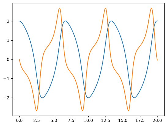
A report is read by its role at a state, as the times were given: out[cx.Trajectory, 'x'], wherever the driver put it. into writes the run into a structure: the computed places it holds, or under a role, each state’s value at the state’s own place, so a history is keyed like the state:

state   = out.into({'x': None, 'y': None})
history = out.into({'x': None, 'y': None}, cx.Trajectory)
state['x'], history['x'].shape

(Array(2.00814976, dtype=float64), (1001,))

The graph is structure only, so one model runs for every \(\mu\): only the inputs change.

And since the run is plain jax, it differentiates through the integrator (diffrax’s adjoint) and jits once per graph:

import equinox as eqx

@eqx.filter_jit
def x_end(mu):
    return flat.run(model, {cx.Inputs: {'mu': mu, 'x(0)': 2.0, 'y(0)': 0.0, 't_s': (0.0, 5.0)},
                            cx.Times: {'x': jnp.linspace(0.0, 5.0, 11)}})['x']

print('x(5) =', x_end(1.0), ' dx(5)/dmu =', jax.grad(x_end)(1.0))

x(5) = -0.8370774355453796  dx(5)/dmu = -1.3140408646792892

An implicit model inside the ODE

The conditional and relational conditional nodes can be combined in the same problem. For example, let’s make the damping term computed by a residual (in this case trivial!)

@flat.rate("y", initial="y(0)", span="t_s")
def accel_z(z, x):
    return z - x

@flat.residual("z")
def damping(z, mu, x, y):
    return z - mu * (1 - x**2) * y

implicit = (flat.declare(vel, accel_z, damping)
            + flat.combine('vdp', (vel.problem, accel_z.problem), cx.OdeCondition)
            + flat.mda())
cx.render_html(implicit, blocks=True)

Newton solves \(z\) inside each rate evaluation, Diffrax integrates around it, and the history is the explicit one:

implicit = (implicit + flat.assign('vdp', cx.Integration(trajectory=True))
            + flat.drive(cx.Newton(), cx.Diffrax(rtol=1e-8, atol=1e-8)))
out = flat.run(implicit, {cx.Inputs: {'mu': 1.0, 'x(0)': 2.0, 'y(0)': 0.0, 't_s': (0.0, 20.0)},
                          cx.Times: {'x': jnp.linspace(0.0, 20.0, 1001)}, cx.Start: {'z': 0.0}})
bool(jnp.allclose(out[cx.Trajectory, 'x'], history['x']))

True