A function that is not jax

cottax never looks inside a node’s implementation: a run just calls it. So a function written in numpy, or a wrapper around a compiled code, is an ordinary node. What has to change is the function itself, because the solvers trace and differentiate whatever they are handed.

This notebook goes through the steps:

1. a plain numpy function, and where it breaks

2. jax.pure_callback, so jax can call it

3. finite differences, so jax can differentiate it

4. the result inside the Sellar problem, solved by Newton and differentiated

5. some notes on cost, and on codes that come with their own derivatives

import jax
jax.config.update('jax_enable_x64', True)   # needed for the finite differences, see section 3
import numpy as np
import jax.numpy as jnp
from jax.flatten_util import ravel_pytree

import cottax.assemblies.jax as cx
from cottax.assemblies.jax import Inputs, Start
flat = cx.flat

1. A numpy function

This stands in for something like a compiled solver. On concrete numbers it works fine, and for a graph without cycles that is run eagerly, that is all you need.

def disc2_host(y_1, z_1, z_2):
    return np.sqrt(np.abs(y_1)) + z_1 + z_2

disc2_host(4.0, 1.0, 2.0)

np.float64(5.0)

Hand it a tracer, though, and it fails:

def show(label, thunk):
    try:
        thunk(); print(f'{label:6s} ok')
    except Exception as e:
        print(f'{label:6s} {type(e).__name__}: {str(e).splitlines()[0][:80]}')

a = (jnp.asarray(4.3), jnp.asarray(1.1), jnp.asarray(2.2))
show('jit',  lambda: jax.jit(disc2_host)(*a))
show('grad', lambda: jax.grad(disc2_host)(*a))

jit    TracerArrayConversionError: The numpy.ndarray conversion method __array__() was called on traced array with 
grad   TracerArrayConversionError: The numpy.ndarray conversion method __array__() was called on traced array with 

np.sqrt on a tracer calls __array__, which raises. Note that you meet this even if you never write jit yourself: a Newton solver differentiates the residual to take a step, so every function inside a solved cycle gets traced.

2. pure_callback

jax.pure_callback runs the function on the host with concrete numpy arrays, and only tells jax the shape of the result. That shape has to be given up front, since jax cannot run the function to find out.

out_shape = jax.ShapeDtypeStruct((), jnp.float64)

def disc2_cb(y_1, z_1, z_2):
    return jax.pure_callback(disc2_host, out_shape, y_1, z_1, z_2, vmap_method='sequential')

show('jit',  lambda: jax.jit(disc2_cb)(*a))
show('grad', lambda: jax.grad(disc2_cb)(*a))

jit    ok
grad   ValueError: Pure callbacks do not support JVP. Please use `jax.custom_jvp` to use callbacks 

Tracing works now, differentiating does not: jax has no idea what the derivative of the callback is. That needs a jax.custom_jvp.

3. Finite differences

There are two ways to write a finite-difference JVP rule, and they behave differently:

mode	rule	calls per JVP	forward mode	reverse mode
directional	(f(x + h v) - f(x)) / h	1	yes	no
jacobian	J @ v, J from one FD sweep	n + 1	yes	yes

Reverse mode needs jax to transpose the rule, which only works if the rule is linear in the tangent v. In directional mode v goes into the callback, so it is not; in jacobian mode it only appears in the matrix product, so it is.

class Tally:
    """Counts how often the host function ran."""
    def __init__(self): self.calls = 0
    def reset(self):    self.calls = 0; return self
    def __repr__(self): return f'{self.calls} call(s)'


def blackbox(fn, out_shape, *, mode='jacobian', tally=None):
    """`fn` made traceable (`pure_callback`) and differentiable (`custom_jvp`, finite differences)."""
    step  = np.sqrt(np.finfo(np.dtype(out_shape.dtype)).eps)

    def call(*args):
        def host(*a):
            if tally: tally.calls += 1
            return fn(*a)
        return jax.pure_callback(host, out_shape, *args, vmap_method='sequential')

    @jax.custom_jvp
    def f(*args):
        return call(*args)

    @f.defjvp
    def _(primals, tangents):
        x, unravel = ravel_pytree(primals)
        v, _       = ravel_pytree(tangents)
        y0         = call(*primals)

        if mode == 'directional':
            nv = jnp.linalg.norm(v)
            h  = step * (1 + jnp.linalg.norm(x)) / jnp.where(nv == 0, 1, nv)
            return y0, (call(*unravel(x + h * v)) - y0) / h

        # one probe per input, so the rule is `J @ v`: linear in v, so jax can transpose it
        h = step * (1 + jnp.abs(x))
        Y = jax.vmap(lambda w: jnp.ravel(call(*unravel(w))))(x[None, :] + jnp.diag(h))
        J = ((Y - jnp.ravel(y0)[None, :]) / h[:, None]).T
        return y0, (J @ v).reshape(out_shape.shape)

    return f

Compared against the same function written in jax:

def disc2_jax(y_1, z_1, z_2):
    return jnp.sqrt(jnp.abs(y_1)) + z_1 + z_2

exact = jax.jacfwd(disc2_jax, argnums=(0, 1, 2))(*a)

for mode in ('directional', 'jacobian'):
    tally = Tally()
    f     = blackbox(disc2_host, out_shape, mode=mode, tally=tally)
    print(mode)
    for name, d in (('jacfwd', jax.jacfwd(f, argnums=(0, 1, 2))),
                    ('jacrev', jax.jacrev(f, argnums=(0, 1, 2)))):
        tally.reset()
        try:
            J   = d(*a)
            err = max(float(abs(p - q)) for p, q in zip(J, exact))
            print(f'   {name}   {tally}   max err {err:.1e}')
        except Exception as e:
            print(f'   {name}   {type(e).__name__}')

directional

   jacfwd   4 call(s)   max err 9.8e-10
   jacrev   RuntimeError
jacobian

   jacfwd   4 call(s)   max err 1.7e-08

   jacrev   4 call(s)   max err 1.7e-08

Some things to note here:

• jacrev with the directional rule fails, because the rule cannot be transposed. The error is not very helpful, so it is good to recognise it.

• A full Jacobian costs n + 1 calls in both modes. The difference is only when they are paid: once per Jacobian, or once per direction.

• n is the number of inputs of this function, not of the whole model. Everything around it is still differentiated exactly by jax, so a large model with one small black box only pays for the box’s own inputs. This is the main reason to wrap the node rather than finite-difference the whole model.

• Use double precision. Finite differences are accurate to about sqrt(eps), which is 1e-8 in double but only 5e-4 in single precision. The function itself has to compute in double as well; casting its result afterwards does not help.

4. In a cottax graph

This is the Sellar problem from the Sellar example, without the optimisation: just the coupled analysis, with discipline 2 replaced by the black box. The same model is declared twice, once with each version of D2, so the two can be compared.

TALLY = Tally()

# built once: a node's function is part of the jit cache key
disc2 = blackbox(disc2_host, out_shape, mode='jacobian', tally=TALLY)

def sellar(d2):
    @flat.function("y_1")
    def D1(x_1, z_1, z_2, y_2):
        return z_1**2 + z_2 + x_1 - 0.2 * y_2

    @flat.function("y_2")
    def D2(y_1, z_1, z_2):
        return d2(y_1, z_1, z_2)

    @flat.function("f")
    def obj(x_1, z_2, y_1, y_2):
        return x_1**2 + z_2 + y_1 + jnp.exp(-y_2)

    declared = flat.declare(D1, D2, obj)
    # cut y_2 where D1 reads it, close the cycle with ^copy.y_2 = y_2 and solve that by Newton
    return declared + flat.fixed_point_cut('y_2', 'D1') + flat.drive(cx.Newton(rtol=1e-10, atol=1e-10))

boxed = sellar(disc2)
plain = sellar(disc2_jax)
cx.render_xdsm_svg(boxed, blocks=True)

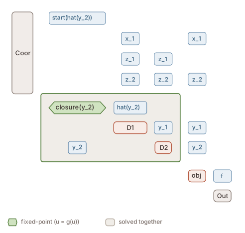
The black box sits in the solved cycle like any other node. The inputs and the Newton’s starting guess for ^copy.y_2 are given by name:

def values(z_1=1.0, x_1=1.0):
    return {Inputs: dict(z_1=z_1, z_2=2.0, x_1=x_1), Start: {cx.copy('y_2'): 1.0}}

TALLY.reset()
out = flat.run(boxed, values())
ref = flat.run(plain, values())
print('black box calls:', TALLY)
for name in ('y_1', 'y_2', 'f'):
    print(f'{name:4s} {float(out[name]):.10f}   jax: {float(ref[name]):.10f}')

black box calls: 17 call(s)
y_1  3.0506762937   jax: 3.0506762937
y_2  4.7466185313   jax: 4.7466185313
f    6.0593572939   jax: 6.0593572939

The Newton converged on a residual that runs through numpy, getting its Jacobian from the finite differences. With only pure_callback, the same solve fails at its first step:

show('solve', lambda: flat.run(sellar(disc2_cb), values()))

solve  ValueError: Pure callbacks do not support JVP. Please use `jax.custom_jvp` to use callbacks 

The gradient through the solve also works. optimistix differentiates the converged solve implicitly, so the finite differences are used twice: in the Newton’s Jacobian, and in the adjoint of the solved cycle.

def objective(model):
    return lambda z_1, x_1: flat.run(model, values(z_1, x_1))['f']

TALLY.reset()
g     = jax.grad(objective(boxed), argnums=(0, 1))(1.0, 1.0)
calls = TALLY.calls
g_ref = jax.grad(objective(plain), argnums=(0, 1))(1.0, 1.0)
print('df/dz_1, df/dx_1 =', [float(v) for v in g], f'  ({calls} calls)')
print('            jax  =', [float(v) for v in g_ref])

df/dz_1, df/dx_1 = [1.6896126157185294, 2.9434964532652685]   (28 calls)
            jax  = [1.689612612212243, 2.943496451317331]

Nothing in cottax itself changed for any of this.

5. Further notes

Reverse mode costs the same as forward mode

mode='jacobian' already gives a VJP, and n + 1 calls is the minimum. One evaluation of f(x + h v) gives a column of J (a JVP). A VJP needs a row, and no perturbation of the inputs gives you one, so you need all n columns. Automatic differentiation avoids this by reading the program; a black box cannot be read. So reverse mode loses its advantage through a black box.

A hand-written custom_vjp costs the same, but then forward mode stops working. Writing the JVP and letting jax transpose it gives you both.

Not storing the Jacobian

In reverse mode J (dense, m x n) is kept in memory until the backward pass. If that is too much, the sweep can be done in the backward pass instead, contracting each column with the cotangent as soon as it is computed:

def bwd(res, ct):
    x, y0 = res
    def body(i, acc):
        h   = step * (1 + jnp.abs(x[i]))
        col = (f(x.at[i].add(h)) - y0) / h
        return acc.at[i].set(jnp.vdot(ct, col))
    return (jax.lax.fori_loop(0, x.size, body, jnp.zeros_like(x)),)

Same number of calls and the same result, with O(n + m) memory instead of O(n m). This is a custom_vjp, so forward mode is lost.

Which mode is best depends on the solver. A dense Newton builds the Jacobian anyway, so jacobian mode costs it nothing extra. A Krylov solver only asks for products J @ v, so there directional mode needs far fewer calls and less memory. jacobian mode inside a Krylov solver is the worst case: n + 1 calls on every product.

jax.ffi: no Python in between

All of the above can be jitted, but each callback still goes back to Python: the compiled program stops, hands buffers to CPython, takes the GIL and continues. That is on the order of a hundred microseconds per call, compared to a few for a direct call.

If the function can be called through a C ABI, jax.ffi makes it a real XLA custom call, about as fast as a native jax operation, and a whole solved cycle then compiles into one XLA program:

jax.ffi.register_ffi_target('disc2', jax.ffi.pycapsule(lib.Disc2), platform='cpu')
jax.ffi.ffi_call('disc2', out_shape, vmap_method='sequential')(y_1, z_1, z_2)

This needs a compiled library (headers from jax.ffi.include_dir()) and a handler per platform. It does not make the function differentiable: ffi_call fails under grad just like pure_callback, and the finite-difference wrapper above goes on top unchanged.

Codes with their own derivatives

Many older simulation codes come with a tangent-linear and/or adjoint routine. These cannot be attached with custom_jvp and custom_vjp together, since a function can only have one of the two. The way to do it is a custom primitive for the linear map v -> J(x) v, with ad.primitive_transposes giving reverse mode and batching.primitive_batchers giving the sweep jacfwd needs. lineax builds its linear_solve_p like this.

the code provides	one JVP	one gradient	forward	reverse
value only	2 calls	n + 1 calls	FD	FD
value + tangent	1 tangent	n tangents	exact	exact
value + adjoint	2 calls	1 adjoint	FD	exact
value + tangent + adjoint	1 tangent	1 adjoint	exact	exact

The same construction works for a fast implementation paired with a slower one written in jax: the fast one computes the values, and jax.jvp / jax.vjp of the jax one give the derivatives. The solve then runs at the speed of the fast implementation and the gradient is that of the jax one, as long as the two really compute the same function.

Summary

• Give the output shape; jax cannot run the function to find it.

• Build the wrapped function once, when declaring the model. It is part of the jit cache key, and a new one on every call means retracing every time.

• Every tangent a rule uses has to go through the linear part. Finite-differencing one argument while passing another through the primitive makes the rule nonlinear again, and transposing it fails.

• Use double precision.

• Jit the run: calling callbacks eagerly is much slower than the jitted call.