Angular discretisation

The equation is now set to hold at \(K\) discreteangles while the integral over the unit sphere is approximated by a discrete quadrature:

\[\int_{S^2} f(\Omega)\, d \Omega = \sum_{\kappa }w_{\kappa} f_{\kappa}\]

The subscript means the evalution at the discrete angle \(\Omega_{\kappa}\) and \(w_{\kappa}\) is the quadrature weight associated with that angle.

The multigroup equation then becomes the following discrete set of coupled PDEs:

\[\left[\Omega_k \cdot \nabla + \sigma_g(\mathbf{r})\right]\psi_{gk}(\mathbf{r}) - \sum_{\ell}\sum_{\tilde{g}}Y_{\ell k } \sigma^s_{\ell g \tilde{g}}(\mathbf{r}) \left[\sum_{\kappa} w_{\kappa} Y_{\ell \kappa } \psi_{\tilde{g}\kappa}(\mathbf{r})\right]= q_{gk}(\mathbf{r}) \ \ \ \forall g,k\]

which is a \(G\times K\) system of 3D partial differential equations.

Let us now introduce the operator notation to simplify the notation. The term in square brackets is:

\[\sum_k w_k Y_{\ell}(\Omega_k) \psi_{gk}(\mathbf{r}) \approx \int_{S^2} Y_{\ell}(\Omega) \psi_{g}(\mathbf{r},\Omega)\,d \Omega = \phi_{g \ell}(\mathbf{r})\]

where \(\phi_{g \ell}(\mathbf{r})\) is the \(\ell\)-th moment of the angular flux in group \(g\). These are the angular moments of the neutron flux — zero is scalar flux, higher are the anisotropic moments. Since the spherical harmonics are orthogonal, they are precisely the expansion coefficients of the projection to a finite spherical harmonic basis:

\[\psi_{g}(\mathbf{r},\Omega) \approx \sum_{\ell }Y_{\ell}(\Omega) \phi_{g\ell}(\mathbf{r})\]

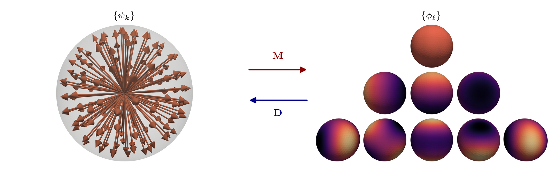
Thus in the discrete ordinates equation, there are two angular descriptions: one is the discrete angles \(k\), and the other is the spherical harmonic expansion coefficients \(\ell\) (naturally arise from scattering).

We now use a free index (not summed over) to mean the full array and implicitly, \(k,\ell\) will indicate angle and moment indices. Dots indicate freely batched indices (i.e., picking out the particular index). Then, we can define the angles-to-moments operator \(\mathbf{M}\), the moments-to-angles operator \(\mathbf{D}\), and the scattering operator \(\mathfrak{s}\) as:

\[\begin{split}\mathbf{M}[a_{\dots k\dots}] &= \sum_{k} w_k Y_{\ell k} a_{\dots k\dots} \label{eq:m_definition_nmd} \\ \mathbf{D}[b_{\dots \ell \dots}] &= \sum_{\ell} Y_{\ell k} b_{\dots \ell \dots} \label{eq:d_definition_nmd}\\ \mathfrak{s}(\mathbf{r})[d_{\dots \tilde{g} \ell\dots }] &=\sum_{\tilde{g}} \sigma^s_{\ell g\tilde{g}} d_{\dots \tilde{g}\ell \dots }\end{split}\]

In other words, the dots imply that

\[\mathbf{M}[a_{gkei}(\mathbf{r})] = \sum_{k}w_k Y_{\ell k }a_{gkei}(\mathbf{r})\]

These \(\mathbf{M}\) and \(\mathbf{D}\) operators convert between the two representations, as in the figure below.

The total transport operator is then (diagonal: only a single \(g,k\))

\[\boldsymbol{\tau}(\mathbf{r}) [f_{gk}] =\Omega_k \cdot \nabla f_{gk} + \sigma_g(\mathbf{r}) f_{gk}\]

The discrete ordinates multigroup transport equation can then be written in a compact form as:

\[\left(\boldsymbol{\tau} - \mathbf{D} \circ \mathfrak{s} \circ \mathbf{M}\right)[ \psi_{gk}(\mathbf{r})]= q_{gk}(\mathbf{r})\]

This is a \(G\times K\) system of 3D PDEs written in a compact operator notation.