Spatial Discretisation

Discontinuous Galerkin is used for the spatial discretisation. This is a generalisation of the finite element methods where discontinuous function values are accepted.

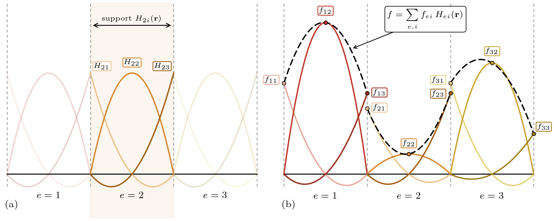
The domain is discretised into \(N\) elements \(e\), and each element has a set of basis functions \(H_{ei}\). In classical finite elements, the basis functions have finite values for multiple elements (e.g. they are a basis function belonging to a node of the mesh), but in discontinuous Galerkin, they are only non-zero within their respective element (finite elements can be obtained by requiring that degrees-of-freedom (DOF) are consistent on each edge node).

The basis functions span a sub-space of \(L^2\), and consequently, an arbitrary function \(f\) within that subspace can be defined by a set of coefficients \(f_{ei}\) as

\[f(\mathbf{r}) = \sum_{e,i} f_{ei} H_{ei}(\mathbf{r})\]

For an interval element, both the basis function and the resulting function approximation are shown below.

Discontinuous Galerkin methods then try to find the best approximation of the solution of the transport equation within that subspace.

Let \(\psi_{gk}\), \(q_{gk}\) be the angular flux for group \(g\) and direction \(k\) within that subspace, and the source term for group \(g\) and direction \(k\), respectively. Multiplying the equation by a basis function \(H_{\epsilon j}\) and integrating over the element \(\epsilon\), requiring the resulting equation to hold for all \(\epsilon,j\) yields the following weak form of the \(G\times K\) transport system:

\[\int_\epsilon \boldsymbol{\tau} \left[\psi_{gk}\right] H_{\epsilon j }\, d V - \int_\epsilon \mathbf{D} \mathfrak{s} \mathbf{M}\left[\psi_{gk}\right] H_{\epsilon j}\, d V = \int_{\epsilon} H_{\epsilon j } q_{gk} \, d V \ \ \ \forall \epsilon,j\]

The first term is currently undefined: it contains a \(nalba \psi_{gk}\) term, which, as \(\psi_{gk}\) is discontinuous, is not defined.

Instead, it can be partially integrated first:

\[\int_{\epsilon}\Omega_k \cdot \nabla \psi_{gk} H_{\epsilon j } \, d V = \int_{\partial \epsilon} H_{\epsilon j }\hat{\psi}_{gk} \Omega_k \cdot \mathbf{n}\, d A - \int_{\epsilon}\psi_{gk} \Omega_k \cdot \nabla H_{\epsilon j}\, d V\]

where the partial integration was performed over the element boundary \(\partial \epsilon\) and \(\mathbf{n}\) is the normal vector along that boundary.

The hat denotes a real ambiguity: the value on the boundary differs between the element \(\epsilon\) and the element connected to it through that boundary.

We now make two additional assumptions

• Elements have straight faces.

• The cross section is constant within an element.

From this point, \(\epsilon,j\) denote the test function (with which the equation is multiplied and integrated) while \(e,i\) are the basis function indices from the expansion of \(\psi_{gk}\). The angular flux is expanded as

\[\psi_{gk}(\mathbf{r}) = \sum_{e,i} \psi_{gkei} H_{ei}(\mathbf{r})\]

and noting that the integration of \(\epsilon\), due to the finite support of the basis functions, only has non-zero contributions for \(e = \epsilon\), the transport operator can be written in a discontinuous-Galerkin form (taking a set of discrete coefficients \(\psi_{gkei}\) as input and returning a set of discrete coefficients defined on \(gk\epsilon j\) as output):

\[\mathbf{T} [\psi_{gkei}] = \sum_{i}\psi_{gk\epsilon i}\int_{\epsilon} H_{\epsilon i}\left[ \sigma_g H_{\epsilon j} - \Omega_k \cdot \nabla H_{\epsilon j}\right]\, d V + \int_{\partial \epsilon} H_{\epsilon j }\hat{\psi}_{gk} \Omega_k \cdot \mathbf{n}\, d A \ \ \left(= T_{gk\epsilon j}\right)\]

which is actually the full \(G\times K \times N \times B\) coefficient set, where \(B\) is the number of basis functions per element.

After we use the assumption that the cross section is constant within an element, it can be taken out of the integral, making the scattering a simple element-wise multiplication. Then, the mass and scattering operators are defined as

\[\begin{split}\mathbf{H}[a_{\dots e i}] &= \sum_{i} a_{\dots \epsilon i}\int_{\epsilon} H_{\epsilon j } H_{\epsilon i} \, d V \label{eq:h_operator_nmd}\\ \mathbf{S}[b_{\tilde{g}\ell \epsilon \dots }] &= \sum_{\tilde{g}} \sigma^s_{\ell g\tilde{g} \epsilon }b_{\tilde{g}\ell \epsilon \dots}\end{split}\]

The dots indicate irrelevant indices, as before. \(\mathbf{H}\) is the mass operator mapping indices \(...ei\) to indices \(...\epsilon j\) (note \(e\) does not shop up because it is only non-zero for \(e = \epsilon\)), and \(\mathbf{S}\) is the scattering operator mapping indices \(\tilde{g}\ell \epsilon ...\) to indices \(g\ell \epsilon ...\) (the constant-cross-section version of \(\mathfrak{s}\)).

The \(\mathbf{H}\) operator commutes with all others except \(\mathbf{T}\) since it only acts on the indices \(i\).

Using these definitions (and the preceding moment and discrete operators) we have the we can write the transport equation (expanding also \(q_{gk}\) in its coefficients) as:

\[\left(\mathbf{T} - \mathbf{D} \mathbf{S} \mathbf{M} \mathbf{H}\right)\left[\psi_{gk ei} \right] = \mathbf{H}[q_{gkei}]\]

giving an operator form of the multigroup, discrete-ordinates, discontinuous-Galerkin discretised transport equation. In principle, this can be used to solve for the coefficients \(\psi_{gkei}\) given a source term \(q_{gkei}\) in a matrix-free fashion, as desired.

Sweep Preconditioning

A major problem is that information only propagates one element in a operator application: a element with 1 with the rest 0 will only transport that value one element per iteration. In a linear mesh, this thus takes \(N\) iterations to propagate information from one end of the mesh to the other. For a \(d\) dimensional mesh, this thus takes \(\propto N^{1/d}\) iterations to propagate information from one end of the mesh to the other.

This does not even include scattering converging, which can also take quite some iterations in highly-scattering regimes. This compounds.

Fortunately, the transport operator admits an inversion that takes roughly the same amount of time as a single operator application. This thus propagates information across the entire mesh in a single iteration. Before showing this sweep, let us show how the operator will look like.

\[\left(\mathbf{I} - \mathbf{T}^{-1} \mathbf{D}\mathbf{S} \mathbf{M} \mathbf{H}\right)[\psi_{gkei}] = \mathbf{T}^{-1}\mathbf{H}[q_{gkei}]\]

Commuting \(\mathbf{H}\) to the right-hand side, we have

\[\left(\mathbf{I} - \mathbf{T}^{-1} \mathbf{H} \mathbf{D}\mathbf{S} \mathbf{M} \right)[\psi_{gkei}] = \mathbf{T}^{-1}\mathbf{H}[q_{gkei}]\]

For scattering, only the moments \(\mathbf{M}[\psi_{gkei]\) are required. Since they are much less numereous than the number of angles, it is advantageous to transform the unknowns the \(\phi_{g\ell ei}\) instead. This requires multiplying both sides by \(\mathbf{M}\):

\[\left(\mathbf{I} -\mathbf{M} \mathbf{T}^{-1} \mathbf{H} \mathbf{D}\mathbf{S} \right)[\phi_{g\ell ei}] = \mathbf{M}\mathbf{T}^{-1}\mathbf{H}[q_{gkei}]\]

or if the source is defined in moment space:

\[\left(\mathbf{I} -\mathbf{M} \mathbf{T}^{-1} \mathbf{H} \mathbf{D}\mathbf{S} \right)[\phi_{g\ell ei}] = \mathbf{M}\mathbf{T}^{-1}\mathbf{H}\mathbf{D}[q_{g\ell ei}]\]

This is the version that can be efficiently solved with any iterative solver.

Transport operator inversion

The transport operator is always diagonal in the \(g,k\) indices; it does not couple these. Obtaining an inverse is thus equal to inverting each \(g,k\) index separately. For brevity, we just drop the indices in this section.

\[T[\psi_{ei}] = \sum_{i}\psi_{\epsilon i}\int_{\epsilon} H_{\epsilon i}\left[ \sigma H_{\epsilon j} - \Omega \cdot \nabla H_{\epsilon j}\right]\, d V + \int_{\partial \epsilon} H_{\epsilon j }\hat{\psi} \Omega \cdot \mathbf{n}\, d A\]

The upwind flux is used as the numerical flux and is defined as:

\[\begin{split}\hat{\psi} = \begin{cases} \sum_{i} \psi_{\epsilon i} H_{\epsilon i} & \Omega \cdot \mathbf{n}(\mathbf{s}) \geq 0 \\ \sum_{i} \psi_{\epsilon(\mathbf{s}) i} H_{\epsilon(\mathbf{s}) i } & \Omega \cdot \mathbf{n}(\mathbf{s}) < 0 \end{cases}\end{split}\]

where \(\epsilon(\mathbf{s})\) is the element connected to \(\epsilon\) through the boundary point \(\mathbf{s}\). In the below mesh and for the particular \(\Omega\) direction, for all boundaries, it is shown which values are used: if the boundary is orange within the element, that value is used, while for inflow boundaries (\(\Omega \cdot \mathbf{n} < 0\)), the value from the neighboring element is used, indicated by the arrow.

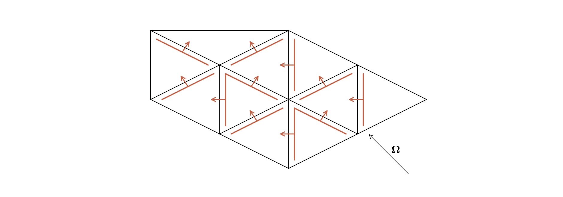
Now, intuitively, if an element has no inflow boundaries, it uses no values from other elements, and thus the solution can be immediately found without reference to such other elements. Then, all elements depending only on that initial element can be solved immediately afterwards, and so on.

This leads to the idea of a dependency graph, shown below.

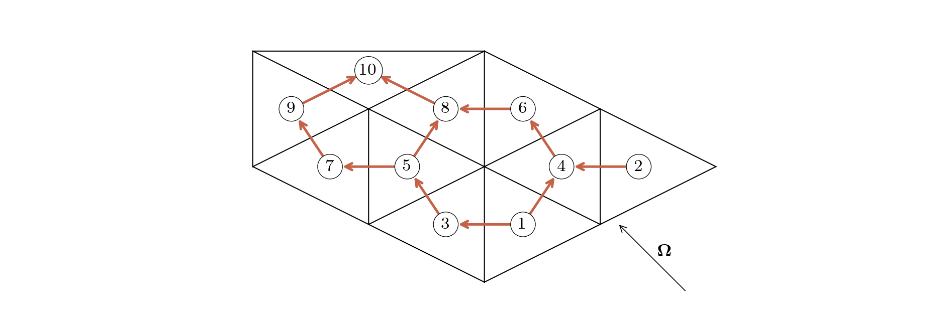
We can use graph theory and its algorithms to find a order in which it can be solved, assuming there are no cycles in the graph (which don’t really seem to happen very often). This topological sorting here leads a simple (non-unique) order:

\[[1,2,3,4,5,6,7,8,9,10] \text{ or } [1, 3, 5,7,9, 2,4,6,8,10]\]

This only requires single-element solves, which due to their very small system size, are comparable to just applying the operator.

Mathematical description

By the straight-faced assumption, each element simply contains a discrete number of straight faces where \(\Omega\cdot \mathbf{n}\) is constant – each face is either outflow or inflow (as in the mesh above). Denote the set of inflow faces for element \(\epsilon\) as \(\beta_{\epsilon}^-\) (and similar for outflow).

The transport operator is then

\[T[\psi_{ei}] = \mathbf{G}_{\epsilon}[\psi_{\epsilon i}] - \sum_{\beta \in \beta^{-}_{\epsilon}} \mathbf{F}_{\epsilon \epsilon(\beta)}[\psi_{\epsilon(\beta) i}]\]

with the single-element matrices defined as

\[\begin{split}\mathbf{G}_{\epsilon}[\psi_{\epsilon i}] &=\sum_i \psi_{\epsilon i } \left[\int_{\epsilon} H_{\epsilon i}\left( \sigma H_{\epsilon j} - \Omega \cdot \nabla H_{\epsilon j}\right)\, d V + \sum_{\beta \in \beta^+_{\epsilon}}|\Omega \cdot \mathbf{n}_\beta|\int_{\beta} H_{\epsilon i} H_{\epsilon j} \, d A \right] \\ \mathbf{F}_{\epsilon \epsilon(\beta)}[\psi_{\epsilon(\beta)i}] &= \sum_{i}\psi_{\epsilon(\beta) i }|\Omega \cdot \mathbf{n}_\beta| \int_{\beta} H_{\epsilon(\beta) i} H_{\epsilon j}\, d A\end{split}\]

For element \(\epsilon\) with all its neighbours known, the solution can be found by solving:

\[\psi_{\epsilon i} = \mathbf{G}_{\epsilon}^{-1}\left[q_{\epsilon i} +\sum_{\beta \in \beta^-_{\epsilon}} \mathbf{F}_{\epsilon \epsilon(\beta)}[\psi_{\epsilon(\beta)i}]\right]\]

This leads to the following algorithm for inverting the transport operator for a right-hand-side \(S_{gkei}\):

Algorithm 1: Transport operator inversion

Setup: Compute topological order \(O_k\) for all angles \(\Omega_k\).

Parallel for \(g = 1, \dots, G\)

Parallel for \(k = 1, \dots, K\)

For \(n = 1, \dots, N\)

Get element in order:

\(e \gets O_k[n]\)

Compute single-element matrix:

\(\mathbf{G}_{gke}\)

Initialize:

\(S_{gkei} \gets 0\)

For \(\beta \in \beta^-_{ek}\)

\(S_{gkei} \mathrel{+}= \mathbf{F}_{ke,e(\beta)} [\psi_{gke(\beta)i}]\)

Compute:

\(\psi_{gkei} \gets \mathbf{G}_{gke}^{-1} [q_{gkei} + S_{gkei}]\)

We can however do better than this: this is fully sequential in all elements, while some elements do not share the same dependency: in the above mesh, element 1 and 2 could be solved in parallel. This is the idea behind level-based parallelism.

Algorithm 2: Transport operator inversion (level-based)

Setup: Compute topological order \(O_k\) and levels \(L_k\).

Parallel for \(g = 1, \dots, G\)

Parallel for \(k = 1, \dots, K\)

For \(l = 1, \dots, L\)

Parallel for \(n \in L_k[l]\)

Get element in order:

\(e \gets O_k[n]\)

Compute single-element matrix:

\(\mathbf{G}_{gke}\)

Initialize:

\(S_{gkei} \gets 0\)

For \(\beta \in \beta^-_{ek}\)

Update:

\(S_{gkei} \mathrel{+}= \mathbf{F}_{ke,e(\beta)} [\psi_{gke(\beta)i}]\)

Compute:

\(\psi_{gkei} \gets \mathbf{G}_{gke}^{-1} [q_{gkei} + S_{gkei}]\)