Energy sets and cross sections

This notebook shows just a few energy sets and how to convert between them. There’s not much else: the energy set is fully defined by the cross sections; picking a right one and obtaining cross sections crucially determines the accuracy of the multi-group simulation.

import jax
import jax.numpy as jnp
jax.config.update("jax_platforms", "cpu")
jax.config.update("jax_enable_x64", True)

Two example energy sets. They are always from high-to-low for this code since this is more logical for downscattering-only problems (you can solve first energy group 0, then 1, etc. instead of going from highest to lowest)

from jax_sn.energy_set.energy_set_examples import vitaminj

energy_set_1 = vitaminj()
energy_set_2 = jnp.logspace(jnp.log10(energy_set_1[0]), jnp.log10(energy_set_1[-1]), 20)

print(energy_set_1)

[1.41907e+07 1.38403e+07 1.34986e+07 1.28403e+07 1.25232e+07 1.22140e+07
 1.16183e+07 1.10517e+07 1.05127e+07 1.00000e+07 9.51229e+06 9.04837e+06
 8.60708e+06 8.18731e+06 7.78801e+06 7.40818e+06 7.04688e+06 6.70320e+06
 6.59241e+06 6.37628e+06 6.06531e+06 5.76950e+06 5.48812e+06 5.22046e+06
 4.96585e+06 4.72367e+06 4.49329e+06 4.06570e+06 3.67879e+06 3.32871e+06
 3.16637e+06 3.01194e+06 2.86505e+06 2.72532e+06 2.59240e+06 2.46597e+06
 2.38513e+06 2.36533e+06 2.34570e+06 2.30693e+06 2.23130e+06 2.12248e+06
 2.01897e+06 1.92050e+06 1.82684e+06 1.73774e+06 1.65299e+06 1.57237e+06
 1.49569e+06 1.42274e+06 1.35335e+06 1.28735e+06 1.22456e+06 1.16484e+06
 1.10803e+06 1.00259e+06 9.61672e+05 9.07180e+05 8.62936e+05 8.20850e+05
 7.80817e+05 7.42736e+05 7.06512e+05 6.72055e+05 6.39279e+05 6.08101e+05
 5.78443e+05 5.50232e+05 5.23397e+05 4.97871e+05 4.50492e+05 4.07622e+05
 3.87742e+05 3.68832e+05 3.33733e+05 3.01974e+05 2.98491e+05 2.97211e+05
 2.94518e+05 2.87246e+05 2.73237e+05 2.47235e+05 2.35177e+05 2.23708e+05
 2.12797e+05 2.02419e+05 1.92547e+05 1.83156e+05 1.74224e+05 1.65727e+05
 1.57644e+05 1.49956e+05 1.42642e+05 1.35686e+05 1.29068e+05 1.22773e+05
 1.16786e+05 1.11090e+05 9.80365e+04 8.65170e+04 8.25034e+04 7.94987e+04
 7.20245e+04 6.73795e+04 5.65622e+04 5.24752e+04 4.63092e+04 4.08677e+04
 3.43067e+04 3.18278e+04 2.85011e+04 2.70001e+04 2.60584e+04 2.47875e+04
 2.41755e+04 2.35786e+04 2.18749e+04 1.93045e+04 1.50344e+04 1.17088e+04
 1.05946e+04 9.11882e+03 7.10174e+03 5.53084e+03 4.30742e+03 3.70744e+03
 3.35463e+03 3.03539e+03 2.74654e+03 2.61259e+03 2.48517e+03 2.24867e+03
 2.03468e+03 1.58461e+03 1.23410e+03 9.61117e+02 7.48518e+02 5.82947e+02
 4.53999e+02 3.53575e+02 2.75364e+02 2.14454e+02 1.67017e+02 1.30073e+02
 1.01301e+02 7.88932e+01 6.14421e+01 4.78512e+01 3.72665e+01 2.90232e+01
 2.26033e+01 1.76035e+01 1.37096e+01 1.06770e+01 8.31529e+00 6.47595e+00
 5.04348e+00 3.92786e+00 3.05902e+00 2.38237e+00 1.85539e+00 1.44000e+00
 1.12300e+00 8.76425e-01 6.82560e-01 5.31579e-01 4.13994e-01 1.00001e-01
 1.00001e-05]

We can visualize these energy sets by simply plotting the energy group boundaries as a function of the index:

import matplotlib.pyplot as plt
plt.stairs(energy_set_2, label="vitaminj")
plt.stairs(energy_set_1, label="vitaminj")
plt.yscale('log')
plt.xlabel("$g$")
_=plt.ylabel("Energy [eV]")

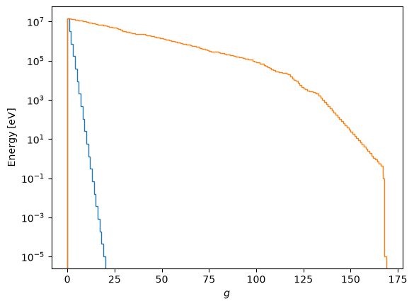
The VitaminJ group structure is not completely logarithmic: it has more resolution in the fast energy regime compared to the resonance regime.

Cross sections

The energy set defines the multigroup equations:

\[\Omega \cdot \nabla \psi_g(\mathbf{r}, \Omega) + \sigma_g(\mathbf{r}, \Omega)\psi_g(\mathbf{r}, \Omega) = \sum_{\ell}\sum_{\tilde{g}}Y_{\ell}(\Omega) \sigma^s_{\ell g \tilde{g}}(\mathbf{r})\int_{S^2}Y_{\ell} (\tilde{\Omega})\psi_{\tilde{g}}(\mathbf{r},\tilde{\Omega}) \,d \tilde{\Omega} \nonumber + q_g(\mathbf{r}, \Omega) \]

where the multigroup cross sections are pre-computed by assuming a guess for the angular flux spectrum:

\[ \sigma_g(\mathbf{r}, \Omega) = \frac{\int \sigma(\mathbf{r}, E) \psi(\mathbf{r}, E , \Omega) \, d E }{\int_g \psi \, d E}\]

\[ \sigma^s_{\ell g \tilde{g}}(\mathbf{r}) = \frac{\int_{S^2}\int_g \int_{\tilde{g}} Y_{\ell}(\tilde{\Omega}) \sigma^s_{\ell}(\mathbf{r}, \tilde{E}\to E)\psi(\mathbf{r}, \tilde{E},\tilde{\Omega}) \, d \tilde{E} \,d \tilde{\Omega}\,d E }{\int_{S^2}\int_{\tilde{g}}Y_{\ell}(\tilde{\Omega}) \psi(\mathbf{r},\tilde{\Omega}, \tilde{E})\, d \tilde{E} \,d \tilde{\Omega}} \]

If a guess is good, the multigroup equation solution will be good; if a guess is bad, the solution will not be accurate to the true solution at all. Also, if a very fine energy group structure is used, the error obtained in wrongly integrating it will not be as large.

Note that after obtaining the cross sections, the energy group boundaries actually do not appear anymore!

In the code

The multigroup cross sections are in this code a simple structure: each element points to a material, which has its array of total cross sections \(\sigma_g\) and the scattering cross section matrices \(\sigma_{\ell g \tilde{g}}\).

An example 2-group water material with first order anisotropic scattering is below:

from jax_sn.domain.cross_sections import CrossSectionData


water = CrossSectionData(
    total = jnp.array([15.2090, 24.4140]),
    scattering = jnp.array([
        [
            [5.5069, 0.0],
            [6.6227, 11.4080]
        ],
        [
            [1.158567, 0.0],
            [1.1234767, 2.4733]
        ]
    ])
)
print(water)

CrossSectionData(total=f64[2], scattering=f64[2,2,2])

The shape of the scattering is [2,2,2]: two for \(l=1\) anisotropic scattering, 2 for two groups outgoing and 2 for two groups ingoing. It is furthermore lower triangular: each incoming group (last index; column) can only scatter to itself or lower energy groups (first index; row).

Normally, you do not hard-code them like this and you obtain them from software which automates the integrals above, including the guess of the flux spectrum.

The OpenMC code can obtain the multigroup cross sections from a simulation in your exact (or similar) geometry, or the NJOY code can assume common spectral shapes.

In FW-CADIS we show how we obtain a breeding-blanket multigroup cross section set from OpenMC.

Comparison between energy sets

After computing a solution to the transport equation, you obtain

\[ \psi_g(\mathbf{r}, \Omega) = \int_g \psi(\mathbf{r}, E, \Omega) \, d E\]

which is the group-averaged flux. This is not directly comparable between energy sets because the boundaries are different.

You can normalise the fluxes by diving by the bin width or lethargy to obtain a visual comparison of the spectrum.

Another option is to map the group-averaged flux to the other energy set using a overlap matrix (basically, how much of the energy group is contained within energy groups of the different energy set). This is exact if the groups do share their boundaries but one is just more coarse.

from jax_sn.energy_set import compute_overlap_matrix